Develop with OctaiPipe#
This short introduction uses OctaiPipe to:
Set up your environment to develop with OctaiPipe.
Write/Load data to and from Influxdb using OctaiPipe modules.
Build a machine learning model that predicts the RUL of assets in an IoT environment.
Register the model to an Azure Storage container.
Evaluate the performance of the model and save the metrics for model monitoring.
Run inference on unseen data points.
We will base our tutorial on the open source C-MAPSS Aircraft Engine Simulator Dataset. We aim to predict the Remaining Useful Life (RUL) of commercial aircraft engines. This dataset was generated with the C-MAPSS simulator. C-MAPSS stands for ‘Commercial Modular Aero-Propulsion System Simulation’ and it is a tool for the simulation of realistic large commercial turbofan engine data. More details can be found in this link.
Below a description of the data in brief
Multivariate time-series data, one for each engine (100 engines)
Each engine starts with some initial wear (unknown), but still in normal condition
At the start of time-series, engine is operating normally
At some point, a fault develops
In the training data, the fault continues growing until system failure
In the test data, the time-series ends prior to system failure
We aim to predict the number of operation cycles before system failure for the test data.
Set up your environment to develop with OctaiPipe#
OctaiPipe is available on a wide variety of platforms including Linux and Mac OS and Windows. Use your preferred IDE such as Jupyter, VSCode, Pycharm, etc. You can create a separate conda environment to have the needed libraries isolated from those installed in other virtual environments. Then, install OctaiPipe and define your environment variable as explained in the OctaiPipe Getting Started Guide page.
In this particular example, we are using Influxdb as a data source to write and load data from the different pipeline steps, so you might need to follow the instructions below to set up your local influxdb instance :
First, make sure you have docker desktop installed.
Second, use the following command to pull the influxdb image and run a local instance on you machine :
docker run -d -p 8086:8086 --name influxdb -v /C/Temp:/var/lib/influxdb2 influxdb:latest
docker run -d - This will run the container as a background process
docker -p 8086:8086 - This will map the Influx port 8086 to your localhost port 8086 so you can access influx locally on http://localhost:8086
--name influxdb - This will name the container
-v /C/Temp:/var/lib/influxdb2 - This will mount the /var/lib/influxdb2 folder in WSL to your local C/Temp folder (make sure you create it :-)) so you can find the data again later
influxdb:latest - This will download the latest version of Influxdb from Influxdb - Official Image | Docker Hub
Once you have run this go to http://localhost:8086 to see where influx is running, and you can set up the ORG and the token that you will need as part of the environment variables setup. Lastly, create an influxdb bucket for each input and output you need.
Now, you are all set to start developing with OctaiPipe !
Write/Load data to and from Influxdb using OctaiPipe modules#
The CMAPS data files are available on our local machine, so we need to load the training data to an influxdb bucket. In a Jupyter notebook or a python file, import the needed libraries, then define the column names of the CMAPSS data. They are as follows:
Machine number - the engine i.d.
Time, in cycles - the operational cycle of the engine
3 operational settings
21 sensors
 columns = ['Machine number', 'Uptime', 'Fuel flow setting', 'Pressure-ratio setting', 'Turbine efficiency setting']
 sensor_measurements = [f'sensor {i}' for i in range(1, 25)]
 columns += sensor_measurements
 sensor_names_mapping = {
'sensor 1': 'Fan inlet thermometer',
'sensor 2': 'LPC inlet thermometer',
'sensor 3': 'LPC outlet thermometer',
'sensor 4': 'LPT inlet thermometer',
'sensor 5': 'LPT outlet thermometer',
'sensor 6': 'Fan inlet pressure',
'sensor 7': 'Fan outlet pressure',
'sensor 8': 'Total pressure in bypass-duct',
'sensor 9': 'Total pressure at HPC outlet',
'sensor 10': 'Physical fan speed',
'sensor 11': 'Engine pressure ratio',
'sensor 12': 'Static pressure at HPC outlet',
'sensor 13': 'Ratio of fuel flow',
'sensor 14': 'Corrected fan speed',
'sensor 15': 'Physical core speed',
'sensor 16': 'Bypass ratio',
'sensor 17': 'Burner fuel-air ratio',
'sensor 18': 'HPT coolant bleed',
'sensor 19': 'LPT coolant bleed',
'sensor 20': 'Demanded fan speed',
'sensor 21': 'Demanded corrected fan speed',
'sensor 21': 'Engine vibration',}
Load and prepare the dataset
df = pd.read_csv('../../cmapss_data/train_FD001.txt', sep=" ", names=columns, index_col=False)
df.drop(columns=['sensor 22', 'sensor 23', 'sensor 24'], inplace=True)
# rename columns names
df.rename(columns=sensor_names_mapping, inplace=True)
The output data, i.e. the RUL, is not provided with the input training data, so some data labelling technique is required. The go-to approach in papers (including this one) is to use piecewise linear labelling. That is, RUL is constant initially and degrades after a certain point. A decision needs to be made on this initial constant, and 125 is often chosen.
We go through the dataframe, select the data for a single engine unit, and compute RUL at each cycle
init_rul = 125
num_units = df['Machine number'].iloc[-1]
outputs = []
for unit in range(1, num_units+1):
    # get the data of the current unit
    unit_df = df.loc[df['Machine number'] == unit]

    # get the end of life i.e. last cycle
    eol = unit_df['Uptime'].iloc[-1]

    # get the start of failure
    sof = eol - init_rul

    # for each operational cycle, compute the RUL based on a piecewise linear function
    for cycle in unit_df['Uptime']:
        output = int(np.piecewise(cycle, [0 <= cycle <= sof, sof < cycle <= eol], [init_rul, eol-cycle]))
        outputs.append(output)

# add RUL to dataframe
df['RUL'] = outputs
Then we convert the uptime in cycles to a timestamp to be able to ingest the data as time series in InfluxDB.
# convert uptime to a timestamp :
timestps = []

max_cycle = int(max(cycle_lengths))
reference_timestamp = datetime.datetime.now() - datetime.timedelta(minutes = max_cycle)

for unit in range(1, num_units+1):
    # get the data of the current unit
    unit_df = df.loc[df['Machine number'] == unit]

    # for each operational cycle
    for cycle in unit_df['Uptime']:
        out =  reference_timestamp + datetime.timedelta(minutes = int(cycle))
        timestps.append(out)

df["timestp"] = timestps

unit = 7
unit_df = df.loc[df['Machine number'] == unit].copy()

# plot RUL vs cycles
plt.figure()
plt.plot(unit_df['timestp'], unit_df['RUL'])

plt.title(f'RUL for engine unit {unit}')
plt.ylabel('RUL')
plt.xlabel('Operational cycle')
plt.show()
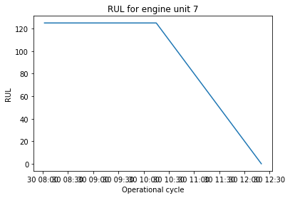
RUL for Engine 7#
Next, we parse the data points and prepare a data dictionary in a format that can be used in InfluxDB.
data = []
# Parse data points
for index, x in df.iterrows():
    # Compute label
    label = x['RUL']
    # Append data point
    data.append(
            {       # Measurement identifier
                    "measurement": 'engine',
                    # Tags - similar in concept to primary key
                    "tags": {
                            "id": x['Machine number']
                            },
                    # Data values
                    "fields": {
                            "Fuel flow setting": float(x['Fuel flow setting']),
                            "Pressure-ratio setting": float(x['Pressure-ratio setting']),
                            "Turbine efficiency setting": float(x['Turbine efficiency setting']),
                            "LPC inlet thermometer": float(x['LPC inlet thermometer']),
                            "LPC outlet thermometer": float(x['LPC outlet thermometer']),
                            "LPT inlet thermometer": float(x['LPT inlet thermometer']),
                            "LPT outlet thermometer": float(x['LPT outlet thermometer']),
                            "Fan inlet pressure": float(x['Fan inlet pressure']),
                            "Fan outlet pressure": float(x['Fan outlet pressure']),
                            "Total pressure in bypass-duct": float(x['Total pressure in bypass-duct']),
                            "Total pressure at HPC outlet": float(x['Total pressure at HPC outlet']),
                            "Physical fan speed": float(x['Physical fan speed']),
                            "Engine pressure ratio": float(x['Engine pressure ratio']),
                            "Static pressure at HPC outlet": float(x['Static pressure at HPC outlet']),
                            "Ratio of fuel flow": float(x['Ratio of fuel flow']),
                            "Physical core speed": float(x['Physical core speed']),
                            "Bypass ratio": float(x['Bypass ratio']),
                            "Burner fuel-air ratio": float(x['Burner fuel-air ratio']),
                            "HPT coolant bleed": float(x['HPT coolant bleed']),
                            "LPT coolant bleed": float(x['LPT coolant bleed']),
                            "Demanded fan speed": float(x['Demanded fan speed']),
                            "Engine vibration": float(x['Engine vibration']),
                            "RUL": float(x['RUL'])

                            },
                    # Timestamp
                    "time": x['timestp']
            }
    )
Finally, we use OctaiPipe’s InfluxDataWriter to load the data to an influxdb bucket as follows:
# You can generate an API token from the "API Tokens Tab" in the UI
url = "http://localhost:8086"
token = "PBmlfEiMPjZZ2bOhR4ns-VViRkL7rktEX7hy3zVxvu9Mt9DMQWc-s7KPGan3uCfSKLL9Wqmammp8-TDYMcn8lQ=="
org = "tdab"
bucket = "cmapss-data"

##############################################################
# Task 2 Repeat local data load using Octaipipe DataWriter
import octaipipe
from octaipipe_core.data.influxdb.influxclient import InfluxClient
from octaipipe_core.data.influxdb.datawriter import InfluxDataWriter

conn = {
        "url": url,
        "token": token,
        "org": org
        }

# Set timeout for INFLUX_CONN_TIMEOUT and INFLUX_READ_TIMEOUT
timeout = (20000, 100000)
# Instantiate InfluxClient
influx_client = InfluxClient(org, url, token,timeout)
# Instantiate DataWriter
data_writer = InfluxDataWriter()
# Use data_writer method
data_writer._write_list_of_dicts(bucket, data)
Build a machine learning model that predicts the RUL of assets in an IoT environment#
Next, we built train a machine learning model to predict the RUL. In order to run the OctaiPipe Model Training Step, you need to provide a yml configuation file as follows
 1name: model_training
 2
 3 input_data_specs:
 4   datastore_type: influxdb
 5   query_type: dataframe
 6   query_template_path: ./configs/data/influx_query.txt
 7   query_values:
 8     start: "2023-01-01T00:00:00.000Z"
 9     stop: "2023-01-01T05:00:00.000Z"
10     bucket: test-bucket
11     measurement: sensors-preprocessed
12   data_converter: {}
13
14 output_data_specs:
15   - datastore_type: influxdb
16     settings:
17       bucket: "cmapss-train"
18       measurement: "dummy"
19   - datastore_type: csv
20     settings:
21       file_path: "./logs/results.csv"
22       append: false
23       delimiter: ","
24
25
26 model_specs:
27   type: lgb_reg_sk
28   load_existing: false
29   name: light_gbm_sklearn
30   model_load_specs:
31     version: '000'
32
33 run_specs:
34   save_results: True
35   target_label: RUL
36   label_type: 'int'
37   grid_search:
38     do_grid_search: True
39     metric: mse
This template allows a guided experience for a more intuitive and faster development experience using
OctaiPipe. The file includes a name, which designates the name of the step, input_data_specs which
specifies what data to be queried through a path to the text file with an influx query to load the data
needed for training:
from(bucket: [bucket])
    |> range(start: [start], stop: [stop])
    |> filter(fn: (r) => r["_measurement"] == "engine")
    |> pivot(rowKey:["_time"], columnKey: ["_field"], valueColumn: "_value")
    |> drop(columns: ["_start", "_stop", "_measurement","id","result","table"])
output_data_specs: This field specifies the destination of the data resulting from the step. In our example,
the data will be written back to an influxdb bucket named “cmapss-train” and a csv file “./logs/results.csv”.
model_specs : This field defines whether a model should be build from scratch or loaded from an existing version.
All blob storage information such as model id, name and version details are provided at this point.
In this example, we train a LightGBM model. OctaiPipe provides a range of models listed under OctaiPipe Models
in the main page.
run_specs : Defines main parameters and configurations under which a certain model will be trained. In our
case, we specify the target label, its type and we use a GridSearch to tune the hyperparameters. We also indicate
the mse as a metric for the GRidSearch.
Use the following command to run the model training step :
1python3 -m octaipipe.pipeline.run_step --step-name model_training --config-path ../configs/data-cmapss/train-config.yml
Register the model to an Azure Storage container#
Some of the advantages of runing a model using OctaiPipe is Reproducibility and Autidibility. In fact, every model is registered and stored on the cloud after every run which makes reproducing the results and auditing models an effortless task. Below, is the trained model file saved to an Azure storage container named machinelearning models. The model file name includes the name of the model as well as a timestamp to differenciate multiple runs.
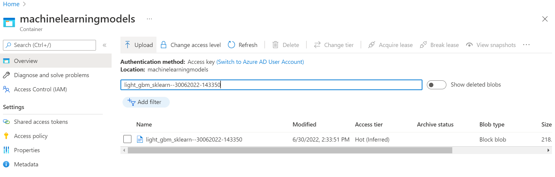
The trained model registered in Azure storage container#
Evaluate the performance of the model and save the metrics for model monitoring#
This step loads the trained model from blob storage then uses the RULEvaluator class to evaluate the remining useful life estimation over the test data. The metrics used for evaluation are those used in RUL literature. It computes the root mean squared error for a set of predictions. It also computes the score which is an asymmetric function that favours early predictions of RUL over late predictions. Results are written back to influxdb under a model-monitoring bucket.
The configuration file for this
 1name: model_evaluation
 2
 3 input_data_specs:
 4   datastore_type: influxdb
 5   query_type: dataframe
 6   query_template_path: ./configs/data/influx_query.txt
 7   query_values:
 8     start: "2023-01-01T00:00:00.000Z"
 9     stop: "2023-01-01T05:00:00.000Z"
10     bucket: test-bucket
11     measurement: sensors-preprocessed
12   data_converter: {}
13
14 output_data_specs:
15   - datastore_type: influxdb
16     settings:
17       bucket: "cmapss-train"
18       measurement: "dummy"
19
20 model_specs:
21   type: lgb_reg_sk
22   load_existing: false
23   name: light_gbm_sklearn
24   model_load_specs:
25     version: 1.3
26
27 run_specs:
28   save_results: True
29   target_label: RUL
30   label_type: 'int'
31   grid_search:
32     do_grid_search: True
33     metric: mse'
34
35 eval_specs:
36     technique: 'RUL' # RUL, anomaly detection etc.
37     eval_final_only:
Use the following command to run the model evaluation step :
1python3 -m octaipipe_core.pipeline.run_step --step-name model_evluation --config-path ../configs/data-cmapss/eval-config.yml
Checkout the model-monitoring bucket to visualize the model performance metrics.
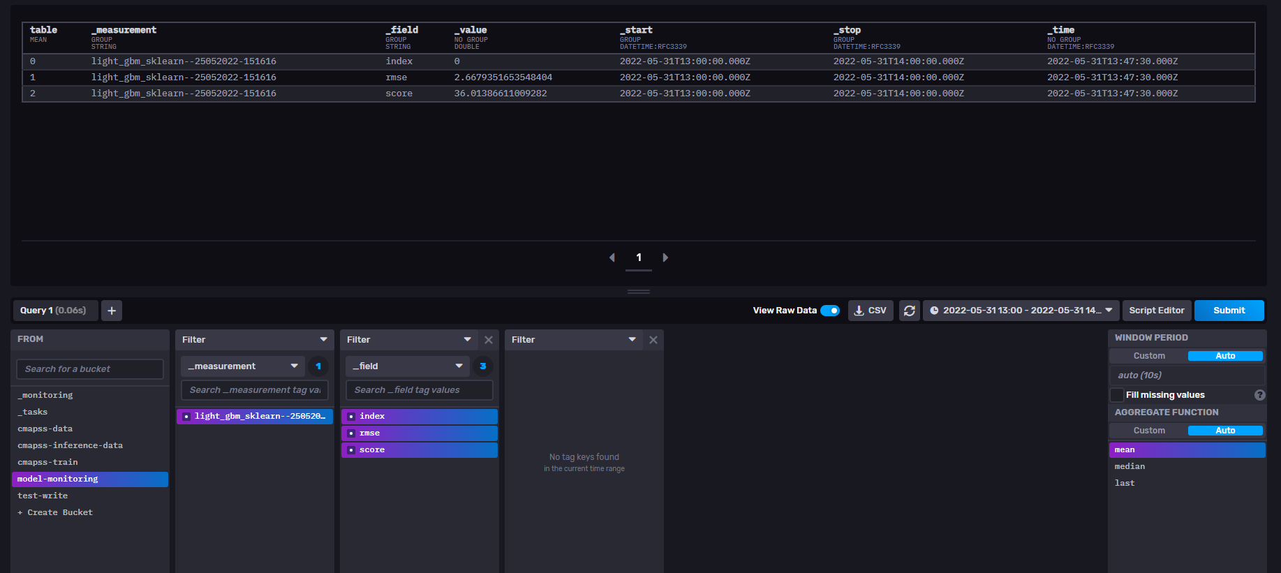
Model Performance Metrics - Output of the Evaluation Step#
Run inference on unseen data points#
We load the inference data to an influx bucket the same way we did for the training data using the InfluxDataWriter. Next, we provide a .YML configuration file that defines the main parameters and configurations under which the inference step will run.
 1name: model_inference
 2
 3 input_data_specs:
 4 datastore_type: influxdb
 5 query_type: 'dataframe'
 6 query_template_path: ../configs/data-cmapss/inference-query.txt
 7 query_values:
 8     start: "2022-06-30T08:00:00Z"
 9     stop: "2022-06-30T11:00:00Z"
10     bucket: cmapss-inference-data
11     measurement: engine
12     tags: {}
13 data_converter: {}
14
15 output_data_specs:
16   - datastore_type: influxdb
17     settings:
18       bucket: "cmapss-train"
19       measurement: "dummy"
20   - datastore_type: csv
21     settings:
22       file_path: "./logs/results.csv"
23       append: false
24       delimiter: ","
25
26 run_specs:
27 prediction_period: 1m
28 save_results: True
The .yml file is referencing a .txt that includes an InfluxDB query to load the inference data :
from(bucket: [bucket])
    |> range(start: [start], stop: [stop])
    |> filter(fn: (r) => r["_measurement"] == "engine")
    |> filter(fn: (r) => r["id"] == "1")
    |> pivot(rowKey:["_time"], columnKey: ["_field"], valueColumn: "_value")
    |> drop(columns: ["_start", "_stop", "_measurement","id","result","table"])
Use the following command to run the model inference step :
1python3 -m octaipipe.pipeline.run_step --step-name model_inference --config-path ../configs/data-cmapss/inference-config.yml
Checkout the output of the inference step in influxDB :
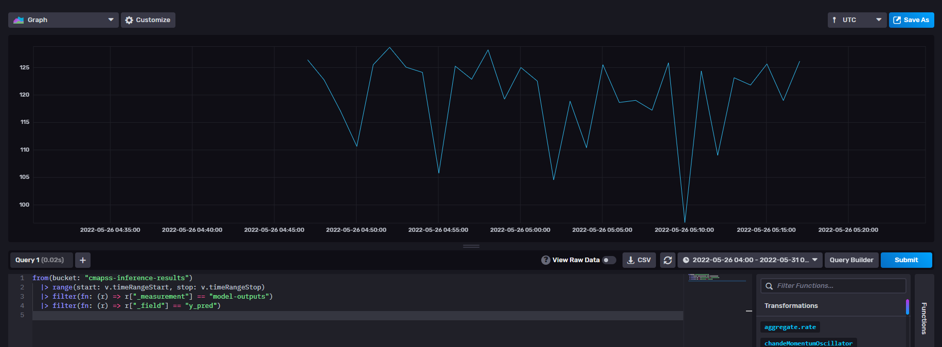
RUL values for unseen data - Output of the Inference Step#