Tutorial - k-FED

This notebook goes through how to run the k-FED algorithm in training and inference using OctaiPipe.

The tutorial does not assume any knowledge of the k-FED algorithm, but it does relate to and builds on the OctaiPipe documentation on k-FED.

This tutorial goes through the following steps:

1. Running k-FED on 3 devices

2. Deploy the resulting model on a fourth holdout device to get cluster predictions

3. Load predictions from holdout device

4. Plot model score of holdout vs. training devices

These steps will show that we can create a model that can identify consistent clusters across training devices. We will also be able to show that this model generalizes to a device that was not included in training.

Assumptions

This tutorial makes a couple of assumptions about your setup that need to be met for the tutorial to run end-to-end without modification.

1. You have 4 devices registered and Available in OctaiPipe

2. The devices have InfluxDB running on them

3. The devices have public IP addresses or can be reached from where this step is run

You can run the tutorial with fewer devices, but you will not be able to run the automatic data setup and results will vary from those we have tested.

If assumption 2 is not met, you will need to adjust all configs in this tutorial to use your data loading and writing methods. Take a look at the data loading and writing utilities for mor information.

If assumption 3 is not met, you will not be able to run the code below which automatically adds data to the devices.

Getting data onto the device

This step adds data to the devices using the add_data_to_devices function. See assumptions above to ensure that you can run this function.

If you cannot run this, the data can be added manually to bucket test-bucket and measurement bearing-{i} where i is the client number.

Note that the function below will assign data from the ./data/client folders in order of the device_ids list, so data from ./data/client_0 will be added to the first device.

We are using the NASA ball bearing dataset which shows failure states of 4 separate ball bearings. We will assume each ball bearing is connected to one OctaiPipe device.

Note that the data for each device falls under different timsestamps. This is to simulate a setting where data loading on each device is not the same.

from load_data_capabilities import add_data_to_devices


device_ids: list = ['device-0', 'device-1', 'device-2', 'device-3']

add_data_to_devices(device_ids)

Defining and Running Federated Learning Workload

Now that the data is on the devices, we can run FL.

Make sure that the correct device IDs are specified in the config ./configs/federated_learning_clustering.yml both in the device_ids list as well as for the input and evaluation data specs.

Running the cells below will import the correct modules, set up and run k-FED using OctaiFL.

import logging

from octaipipe.federated_learning.run_fl import OctaiFL


logging.basicConfig(level=logging.INFO, format='%(message)s')

config_path = './configs/federated_learning_clustering.yml'

octaifl = OctaiFL(config_path=config_path,
                  deployment_name='FL demo deployment',
                  deployment_description='Deployment for Federated Learning demo')

strategy = {'experiment_description': 'FL training of kmeans model'}
octaifl.strategy.set_config(strategy)


octaifl.run()

Model Deployment to holdout device

Next we deploy the model to the holdout device to get predictions from it.

In order to use the correct model, follow the link to the experiment page from the k-FED training run. Note the model version number and in the file ./configs/inference_config.yml, adjust the model version number in the model_specs.

from octaipipe.deployment import deploy_to_edge


deploy_to_edge(config_path='./configs/deployment.yml')

Next we down the deployment to ensure we do not leave an exited container on the device.

Take the deployment ID from the output of the cell above and set it in the down_deployment function.

NOTE: Make sure to give the deployment a minute or two to finish running, otherwise no predictions will have been made.

from octaipipe.deployment import down_deployment


logging.basicConfig(level=logging.DEBUG, format='%(message)s')

down_deployment('INSERT_DEPLOYMENT_ID')

Test predictions against ground truth labels

Next we load the predictions from the holdout device and compare them to the scores from the other devices.

In the load_predicted_data function below, add the InfluxDB org, url and token of the holdout device.

from load_data_capabilities import load_predicted_data, get_training_scores


y_pred = load_predicted_data(INFLUX_ORG='',
                             INFLUX_URL='',
                             INFLUX_TOKEN='')

Next, we load the ground truth labels of the holdout device and calculate the mutual information score. This is a score that goes from 0 to 1, and notes co-occurance of two series. A higher score means greater co-occurance.

It is worth noting that in most real-life scenarios, you will not have ground truth labels for an unsupervised learning task. This is simply an example evidencing that the clustering algorithm can generalize.

import pandas as pd


y_true = pd.read_csv('./data/client_3/y.csv')
y_true = y_true['0'].values

from sklearn.metrics import adjusted_mutual_info_score


score = adjusted_mutual_info_score(y_true, y_pred)
scores = get_training_scores(score)
print(f'Adjusted mutual info score: {score}')

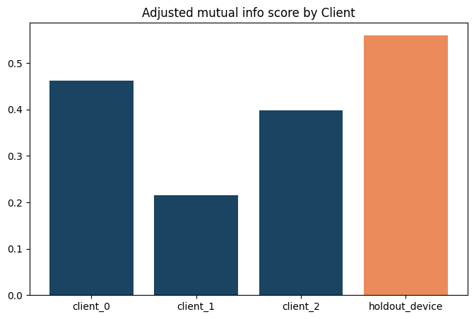
Adjusted mutual info score: 0.5587905638718519

Plot scores per device

Now, we use the score we got from the cells above and plot it against previously known scores from the devices used in training (these scores are retrieved from the get_training_scores function above).

The first three bars are the devices included in training and the holdout device is orange.

import matplotlib.pyplot as plt


clients = list(scores.keys())
score_values = list(scores.values())
colors = ['#1a4462', '#1a4462', '#1a4462', '#eb8b5c']

plt.figure(figsize=(8, 5))
plt.bar(clients, score_values, color=colors)
plt.title('Adjusted mutual info score by Client')

plt.show()

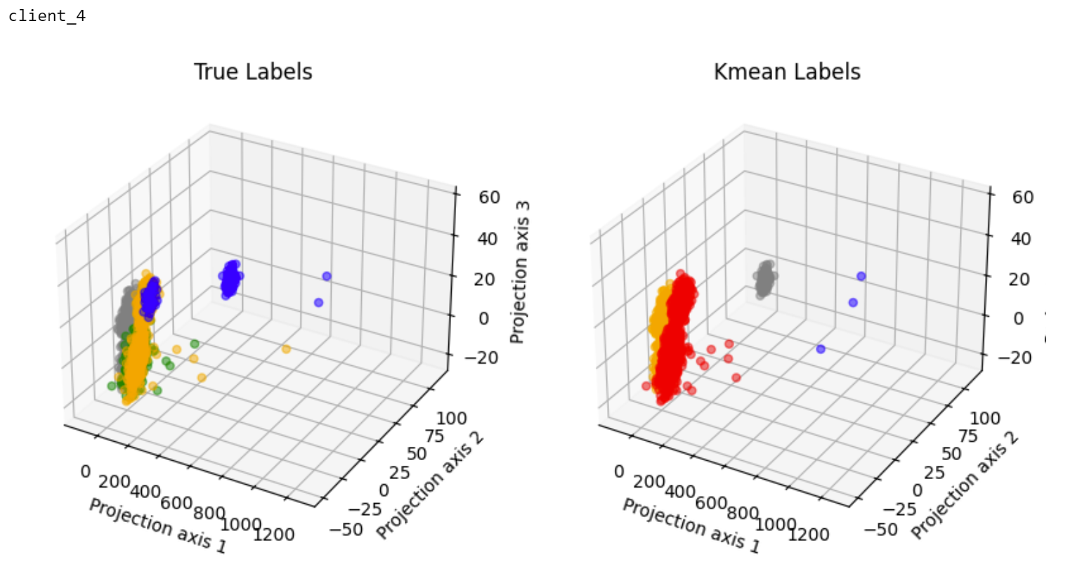
Clusters visualized in 3D space

We also include a plot visualizing the clusters of the holdout device true labels (left) and k-FED predictions (right).

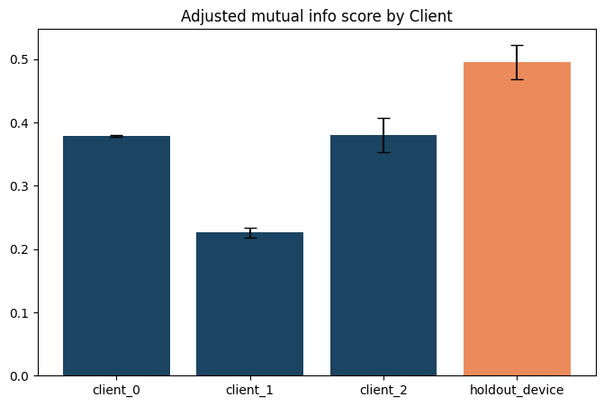
Plotting with error bars

Finally, we include a plot of mutual information scores with the mean score of 10 runs for each device. We also include error bars showing SEM.

import pandas as pd
import matplotlib.pyplot as plt

df = pd.read_csv('./data/record_scores.csv')
means = df.mean()
sem = df.sem()

colors = ['#1a4462', '#1a4462', '#1a4462', '#eb8b5c']

plt.figure(figsize=(8, 5))
plt.bar(means.index, means.values, yerr=sem.values, capsize=5, color=colors)
plt.title('Adjusted mutual info score by Client')
plt.show()