Feature Engineering Step

To run locally: feature_engineering

Feature engineering is used to transform raw data into a new set of features, for a few reasons:

Data reduction - feature engineering allows us to capture the important properties of the data whilst removing the redundant information or noise. This results in a feature space smaller than the original dataset and in turn means faster model training.

Improved performance - feature engineering allows us to construct new features that can better explain the relationship between our inputs and outputs.

Simpler models - because the relationship between input and output can be better explained, simpler models may also be trained, meaning faster training times and potentially better explainability.

In this pipeline step, from the time series data, various time-domain, frequency-domain, and time-frequency-domain features are extracted over sliding windows. Moreover, lag features are generated and features are re-scaled. The user can also perform a train-validation-test split of the resulting features.

The following are examples of config files respectively for running the step once and periodcally, together with descriptions of its parts.

Config example for running the step once

name: feature_engineering

input_data_specs:
  datastore_type: influxdb
  query_type: dataframe
  query_template_path: ./configs/data/influx_query.txt
  query_values:
    start: "2020-05-20T13:30:00.000Z"
    stop: "2020-05-20T13:35:00.000Z"
    bucket: sensors-raw
    measurement: cat
    tags: {}
  data_converter: {}


output_data_specs:
  - datastore_type: influxdb
    settings:
      bucket: test-bucket-1
      measurement: testv1-fe


run_specs:
  save_results: True
  target_label: accel_x
  feature_lagging:
    to_lag: True
    num_previous_vals: 3 # number of previous values to concat to each row
  train_val_test_split:
    to_split: True # should the feature space be split up
    split_ratio:
      training: 0.6
      validation: 0.2
      testing: 0.2

feature_specs:
  feature_domain: raw_data # feature domain type - raw_data, time, freq, time-freq
  features:
    - "minimum"
    - "maximum"
    - "variance"
  sliding_window:
    length: 20 # number of samples in the sliding window
    overlap: 0.8 # overlap of windows as a proportion
  normalise_features: False # should the features be scaled

Config example for running the step periodically

name: feature_engineering

input_data_specs:
  datastore_type: influxdb
  query_type: dataframe
  query_template_path: ./configs/data/influx_query_periodic.txt
  query_values:
    start: 2m
    bucket: live-metrics
    measurement: live-processed
    tags: {}
  data_converter: {}

output_data_specs:
  - datastore_type: influxdb
    settings:
      bucket: live-metrics
      measurement: live-fe

run_specs:
  save_results: True
  run_interval: 10s
  target_label: accel_x
  feature_lagging:
    to_lag: True
    num_previous_vals: 3 # number of previous values to concat to each row
  train_val_test_split:
    to_split: True # should the feature space be split up
    split_ratio:
      training: 0.6
      validation: 0.2
      testing: 0.2

feature_specs:
  feature_domain: raw_data # feature domain type - raw_data, time, freq, time-freq
  features:
    - "minimum"
    - "maximum"
    - "variance"
  sliding_window:
    length: 20 # number of samples in the sliding window
    overlap: 0.8 # overlap of windows as a proportion
  normalise_features: False # should the features be scaled

Input and Output Data Specs

input_data_specs and output_data_specs follow a standard format for all the pipeline steps; see Octaipipe Steps.

Run Specs

This section specifies some high-level options for the step.

run_specs:
 save_results: True
 run_interval: 10s
 target_label: 'RUL'
 feature_lagging:
     to_lag: True
     num_previous_vals: 3
 train_val_test_split:
     to_split: True
     split_ratio:
         training: 0.6
         validation: 0.2
         testing: 0.2

Level 1	Level 2	Level 3	Type/Options	Description
save_results			bool	if False, the step is flushed without saving any of the outputs, only use for testing.
run_interval			str	if this key is present, the step will be run periodcally at the specified interval. Value is given in minute (e.g. 2m), or in second (e.g. 10s).
target_label			str	Label of the column imported that is going to be the target variable. It will excluded from the feature engineering, but will be saved together with the engineered features
feature_lagging	to-lag		bool	Option to use feature lagging, i.e. concatenating several rows of features into one row with (t-n) suffix. Only used in time-series problems
	num_previous_vals		int	Number of timestamps to use in single ro
train_val_test_split	to_split		bool	if True, the whole transformed dataset will be split into three sections according to the ratios below and saved with corresponding tags
	split_ratio	training	float	Ratios defining the data split into training, validation and test, you can then use the tags for model training step subset. Note! The three floats must add up to 1.0
		validation	float
		testing	float

Feature Specs

This section provides control of the specifics of the feature engineering process to be undertaken.

feature_specs:
 feature_domain: time
 features:
     - 'minimum'
     - 'maximum'
     - 'variance'
 sliding_window:
     length: 20
     overlap: 0.8
 normalise_features: false

The first thing you have to choose is wether you want to extract time-based, frequency-base or frequency-time-based features.

Time Domain

Time-domain feature engineering looks to extract descriptive statistical properties directly from the time-series signal. By extracting individual properties over a window of data, the most useful information can be retained whilst the data size is reduced.

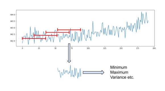
To do this, the approach is shown above. A sliding window is passed over the signals, extracting features as it goes. The sliding window has two properties: (1) length and (2) overlap. The length of the window is determined by how far back useful information remains. The overlap determines how many new samples we want in the feature space.

The step for moving through the data is computed with:

step = int(window_length-(window_overlap*window_length))

e.g. a window length of 10 with 50% overlap would give a step of 5. The for loop to move through the dataframe df is then:

for i in range(window_length, len(df)+step, step):

and the window of data is:

x_win = df.iloc[i-window_length:idx, :].to_numpy()

From this window, the features currently defined in the framework that can be extracted are:

Feature name	Description
minimum	Smallest value in the signal.
maximum	Largest value in the signal.
variance	Variability of the signal from its mean.
root_mean_square	Average power of the signal.
skewness	Symmetry of the signal.
kurtosis	How tail-heavy the signal distribution is.
energy	Energy of the signal as given by Parseval’s theorem.
slope_sign_changes	The total number of times the slope of the signal changes sign. An approximation of the frequency of the signal (higher frequency signals will change slope more).
waveform_length	Cumulative length of the signal.
shannon_entropy	Uncertainty of the signal.

These features can be on different scales of magnitude, which can hinder training for certain types of learning algorithm. It can therefore be specified in the config file to normalise the features following extraction, which is done with scikit-learn’s MinMaxScaler.

Config Arguments:

feature_domain: time
features:  # list of features from above
sliding_window:
    length:  # length of the sliding window in samples
    overlap:  # overlap of the sliding window as a proportion (between 0.0 and 1.0)
normalize_features:  # if True, features are scaled following the feature engineering

Frequency Domain

There also exists useful information in how the frequency components of time-series signals change over time that can be used as features. Signals are transformed from time-domain to frequency-domain with the Fourier transform (FT). The FT assumes the signals to be stationary (parameters don’t change over time) and as such the transform has zero time resolution, i.e. it can’t detail when different frequencies occurred in the signal.

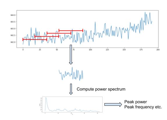
The most basic solution is the short-time FT (STFT). The STFT splits the signal into fixed-sized windows, and in each window computes the FT. This windowing procedure is carried out as described in the section above. The difference is that when the window is obtained i.e.

x_win = df.iloc[i-window_length:idx, :].to_numpy()

The power spectral density (PSD) estimate of the window is then computed with SciPy’s welch function:

psd, freqs = welch(x_win, fs=fs, window='hann', axis=0, nperseg=len(x_win)//2)

The PSD describes how the power of the signal is distributed over the frequencies, and is typically used over the FT for feature engineering. The PSD is estimated from the discrete FT (DFT) with the periodogram, computed as the squared magnitude of the DFT. Welch’s PSD estimate improves upon the periodogram by computing the modified periodogram, which uses a window function to reduce spectral leakage, in overlapping windows (within the current STFT window) and taking the average, which reduces variance in the estimate.

The Hann window function is kept simply as the default. The nperseg=len(x_win)//2) argument means that for a window of 50 samples, it is split into segments of 25 samples. The default argument of noverlap = nperseg // 2 is kept and as such, the window would be split into segments of 25 samples, with an overlap of 12 samples.

From the power spectrum of each window, the following features can be extracted:

Feature name	Description
peak_power	Largest power value
peak_frequency	Thre frequency at which peak power occurs
mean_frequency	Sum of the preduct of the power spectrum and frequencies divided by the sum of the power spectrum
median_frequency	The frequency that splits the power spectrum into two regions of equal total power
spectral_entropy	Measure os spectral power distribution
mean_power_q1	Mean power of the first quater of the signal
mean_power_q2	Mean power of the second quarter of the signal
mean_power_q3	Mean power of the third quarter of the signal
mean_power_q4	Mean power of the fourth quarter of the signal

Note

The bottow four features are an alternative to directly using the PSD coefficients to cut down on the number of features

Config Arguments:

feature_domain: freq
features:  # list from above
sampling_frequency:  # frequency the signal was sampled at, in Hz
sliding_window:
  length:  # length of the sliding window in samples
  overlap:  # overlap of the sliding window as a proportion (between 0.0 and 1.0)
normalize_features:  # if True, features are scaled following the feature engineering

Time-Frequency Domain

Note

Useful link: Link A guide for using wavelet transform in ML

The STFT has fixed window sizes, and in turn fixed time-frequency resolution. If the signal shows slowly fluctuating properties, a longer window is needed to capture this, and there is good frequency resolution but poor time resolution. Conversely, if the signal has rapidly fluctuating properties, a short window is needed, that has good time resolution but poorer frequency resolution. This means there is always a trade-off with the STFT between time and frequency resolution. To overcome the limitations of the STFT, the Wavelet transform was developed. The Wavelet transform uses short windows for larger frequencies, and longer windows for smaller frequencies. Wavelets are small, finite oscillations, localised in time. The wavelet moves along the signal, where the two are convolved. The wavelet is then scaled, and the process repeated. Higher scaled (i.e. longer) wavelets analyse smaller frequencies, and smaller scaled wavelets analyse higher frequencies. The output of the continuous wavelet transform is 2D; both time and frequencies and as such frequencies are highly localised in time, without the trade-off of the STFT.

Computation of the CWT for each signal is with the Link PyWavelets library

coefs, freqs = pywt.cwt(data=signal, scales, wavelet)

scales are the scaling factors and can be converted to frequencies with f = scale2frequency(wavelet, scale)/sampling_period. Setting the scales depends on the frequencies to be analysed within the signal.

wavelet is the type of wavelet function to be used. The choice of wavelet depends on the properties of the signal being analysed and some experimentation is needed to find the best one.

For feature engineering, the scalogram is used, given by the absolute value of the CWT i.e.:

scalogram = np.absolute(coefs)

The shape of coefs is len(scales) x len(signal) and so the scalogram is transposed to have timesteps as rows.

Config Arguments:

feature_domain: time-freq
sampling_period:  # 1/sampling_frequency, in seconds
wavelet:  # choice of wavelet from ``pywt.families()``
scales:
    low_scale_factor:  # smallest scale factor in the CWT
    high_scale_factor:  # largest scale factor in the CWT
    step:  # size of step when creating scale factors between low and high
normalise_features:  # if True, features are scaled following the feature engineering