Evaluating k-FED#
Introduction#
OctaiPipe has developed a set of features to help explain and evaluate k-FED models trained using the platform. These tools can help with a number of use-cases, such as labeling data, finding outliers in data, or grouping devices.
Evaluation metrics collected by OctaiPipe#
Metrics always collected#
Local WCSS for local data and local cluster (K-means)
Global WCSS for local cnetroids and global clusters (K-means)
Global silhouette score for local centroids and global cluster (Silhouette score)
Inertia of global k-FED model (K-means)
Metrics requiring ground truth labels#
Additional data collected#
Proportion of test data on each device belonging to each global cluster (called global cluster proportions)
Local cluster centroids for the test data
Global cluser centroids
Inspecting metrics for k-FED#
To view saved metrics and other data for a k-FED model, the following functions can be run
from the octaipipe.explainability module, e.g. from octaipipe import explainability
and then explainability.get_explainability_record_by_model_id. Each function takes
the model ID as input. These functions are explained in more detail in the Python Interface section.
get_explainability_record_by_model_id- gets full record for model with no detailsget_global_metrics_by_model_id- gets global metrics recorded for modelget_local_metrics_by_model_id- get local metrics calculated for each deviceget_global_cluster_proportions_by_model_id- gets proportions of test data beloning to each global cluster on each deviceget_global_centroids_by_model_id- gets global centroids and saves to~/model_metrics/{model_id}/global_centroids/centroid_{global_centroid_id}.npyget_local_centroids_by_model_id- gets local centroids and saves to~/model_metrics/{model_id}/local_centroids/centroid_{local_centroid_id}.npyget_local_centroid_distances_by_model_id- shows Euclidean distance between local centroids and global centroids
Visualizing k-FED in OctaiPipe#
OctaiPipe comes with some pre-built visualization functionalities for k-FED models.
The following plotting functions can be imported from octaipipe.visualization.kfed:
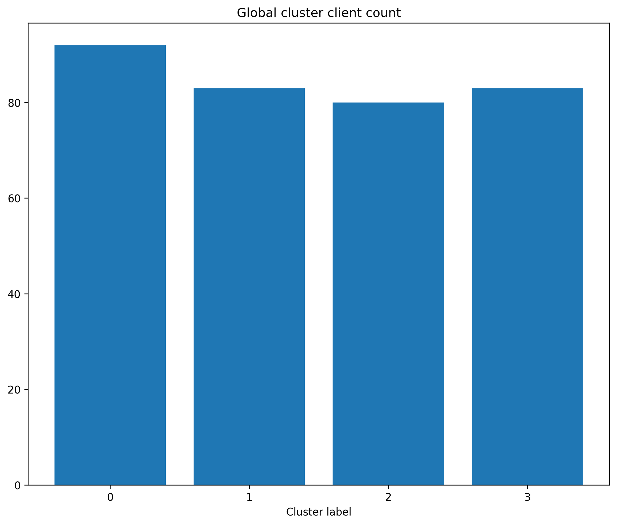
Number of clients with data in each global cluster#
Function: plot_cluster_client_count
This plots the number of local clients that have data belonging to each of the global clusters.
- octaipipe.visualization.kfed.plot_cluster_client_count(model_id: str, cluster_label_map: dict = {}, barplot_args: dict = {}, savefig: bool = False, output_path: Optional[str] = None, figsize: tuple = (10, 8), plot_title: str = 'Global cluster client count', xlabel: str = 'Cluster label', ylabel: str = 'Client count')#
Bar plot showing the number of clients that a cluster is present in.
- Parameters:
model_id (str) – model to generate plot for
cluster_label_map (dict) – mapping between cluster assignment and label
barplot_args (dict, optional) – Any arguments to hand to pyplot.bar as kwargs. Defaults to {}.
savefig (bool, optional) – Save figure to file. Defaults to False.
output_path (str, optional) – If savefig is True, must be set to path to save to.
figsize (tuple, optional) – Defaults to (10, 8).
plot_title (str, optional) – Defaults to ‘Global cluster client count’.
xlabel (str, optional) – Defaults to ‘Cluster label’.
ylabel (str, optional) – Defaults to ‘Cluster count’.
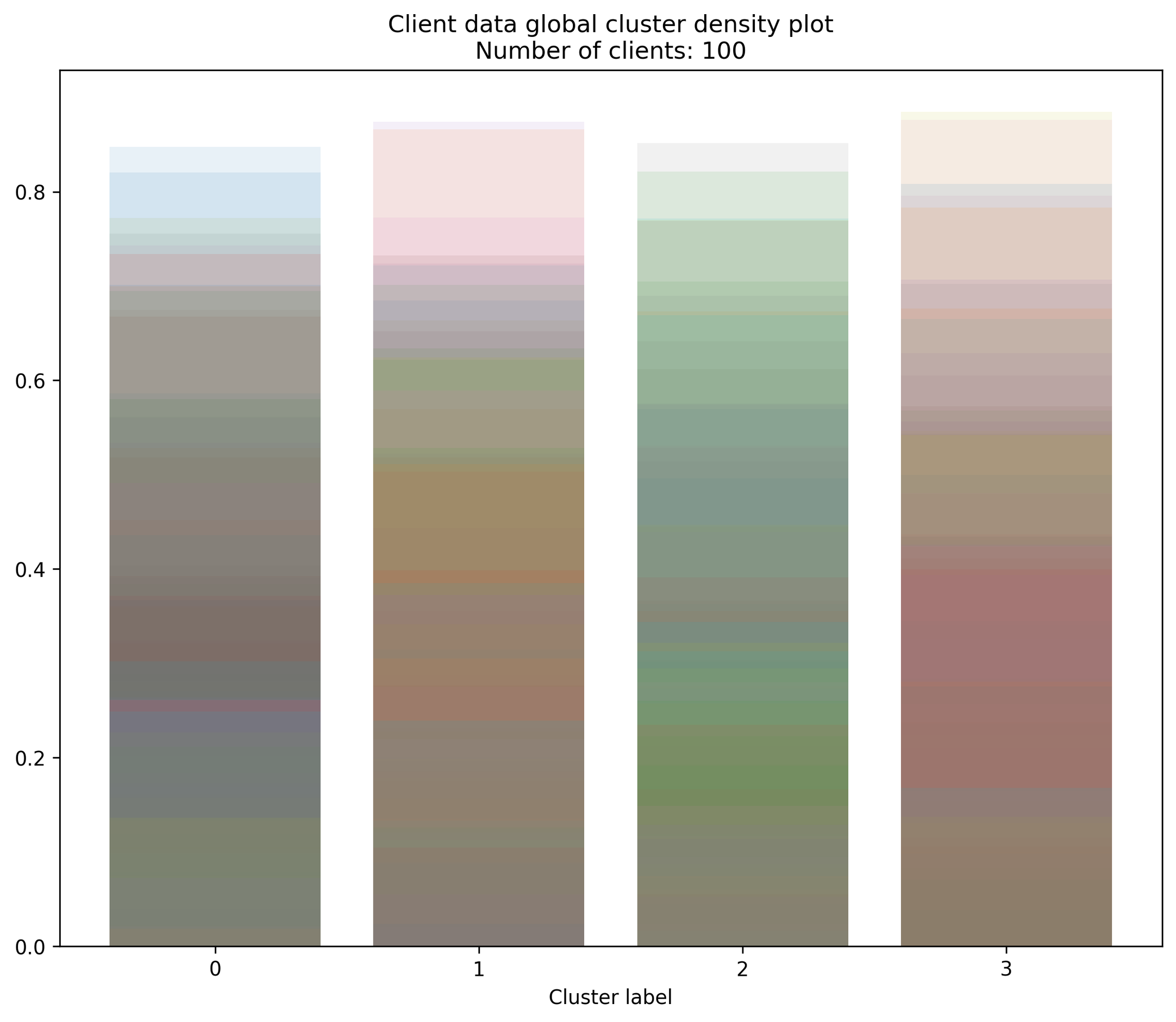
Proportion of data in each global cluster for each client#
Function: plot_client_cluster_frac
This plots the proportion of local data points of each client that is in each global cluster. The bar chart shows the density of clients with a specific proportion of their data in a global cluster. Each device has its own color of transparent bar that are overlayed on top of one another. This means the areas that are most filled in have the highest density of global cluster proportions.
- octaipipe.visualization.kfed.plot_client_cluster_frac(model_id: str, cluster_label_map: dict = {}, barplot_args: dict = {'alpha': 0.1}, savefig: bool = False, output_path: Optional[str] = None, figsize: tuple = (10, 8), plot_title: str = 'Client data global cluster bar plot', xlabel: str = 'Cluster label', ylabel: str = 'Proportion of client data in global cluster')#
Bar plot for global client cluster
- Parameters:
model_id (str) – model to generate plot for
cluster_label_map (dict) – mapping between cluster assignment and label
barplot_args (dict, optional) – Any arguments to hand to pyplot.bar as kwargs. Defaults to {‘alpha’: 0.1}.
savefig (bool, optional) – Save figure to file. Defaults to False.
output_path (str, optional) – If savefig is True, must be set to path to save to.
figsize (tuple, optional) – Defaults to (10, 10).
plot_title (str, optional) – Defaults to ‘Client data global cluster density plot’.
xlabel (str, optional) – Defaults to ‘Cluster label’.
ylabel (str, optional) – Defaults to ‘Cluster number’.
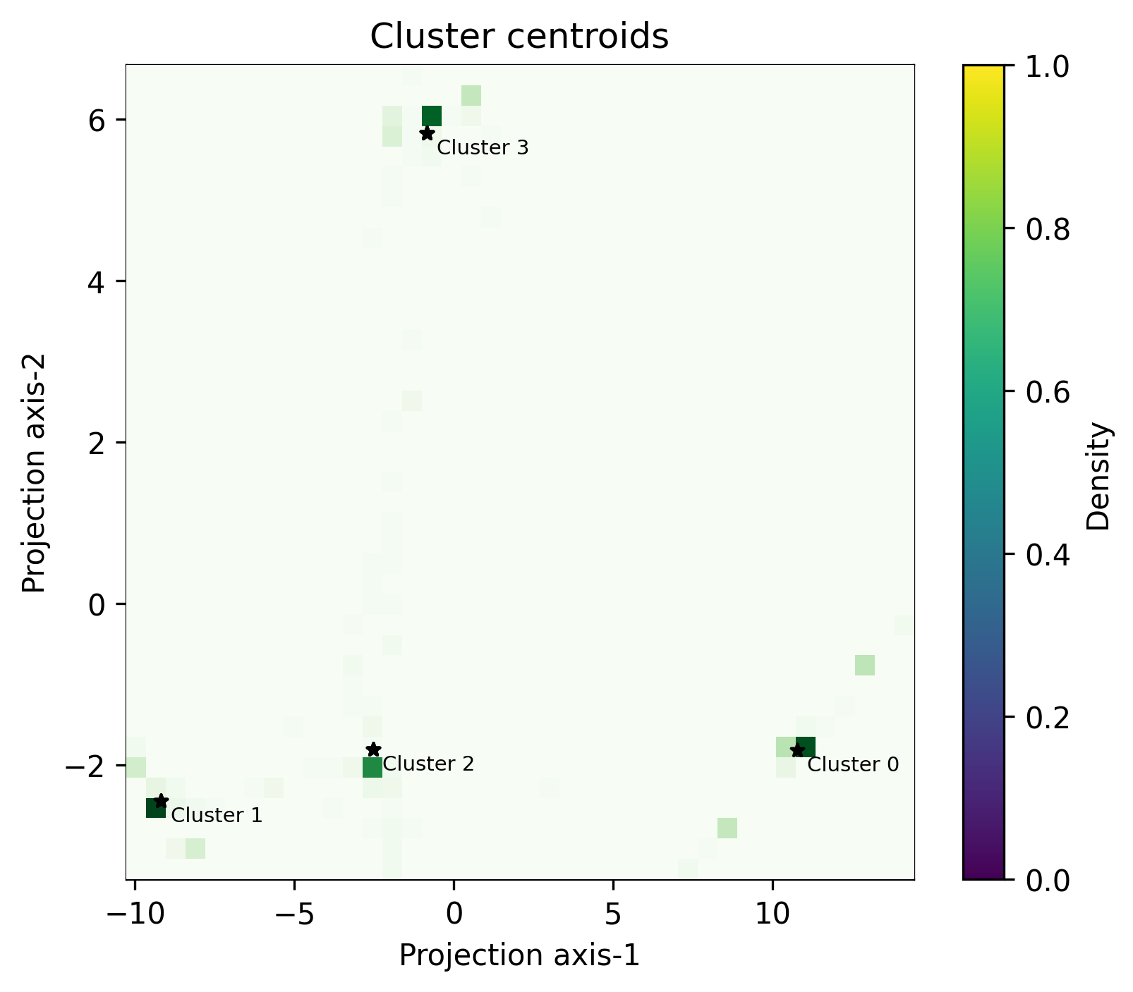
Plot centroids in 2D heatmap#
Function: plot_centroids_2d_heatmap
Global centroids plotted with the local centroids represented in a heatmap around them. The feature space has been reduced to 2 dimensions using PCA.
- octaipipe.visualization.kfed.plot_centroids_2d_heatmap(model_id: str, refresh_centroids: bool = True, cluster_label_map: dict = {}, bins: int = 40, savefig: bool = False, output_path: Optional[str] = None, heatmap_args: dict = {'aspect': 'auto', 'cmap': 'Greens'}, global_plot_args: dict = {'c': 'black', 'marker': '*', 's': 20}, figsize: tuple = (6, 5), plot_title: str = 'Cluster centroids', xlabel: str = 'Projection axis-1', ylabel: str = 'Projection axis-2', annotate_fontsize: int = 7)#
Heatmap plot for local and global centroids in 2d-PCA-reduced space.
- Parameters:
model_id (str) – model ID to plot the centroids for.
refresh_centroids (bool) – whether to get centroids from blob storage regardless of whether they are present on machine. Defaults to True
cluster_label_map (dict) – mapping between cluster assignment and label
bins (int, optional) – heatmap bins. Defaults to 40.
savefig (bool, optional) – Save figure to file. Defaults to False
output_path (str, optional) – If savefig is True, must be set to path to save to.
heatmap_args (dict, optional) – plot args for local centroids heatmap. Defaults to {‘cmap’: ‘Greens’, ‘aspect’: ‘auto’}.
global_plot_args (dict, optional) – plot args for global centroids. Defaults to {‘c’: ‘black’, ‘s’: 10, ‘marker’: ‘*’}.
figsize (tuple, optional) – Defaults to (6, 5).
plot_title (str, optional) – Defaults to ‘Cluster centroids’.
xlabel (str, optional) – Defaults to ‘Projection axis-1’.
ylabel (str, optional) – Defaults to ‘Projection axis-2’.
annotate_fontsize (int, optional) – font size of global centroid annotation. Defaults to 7.
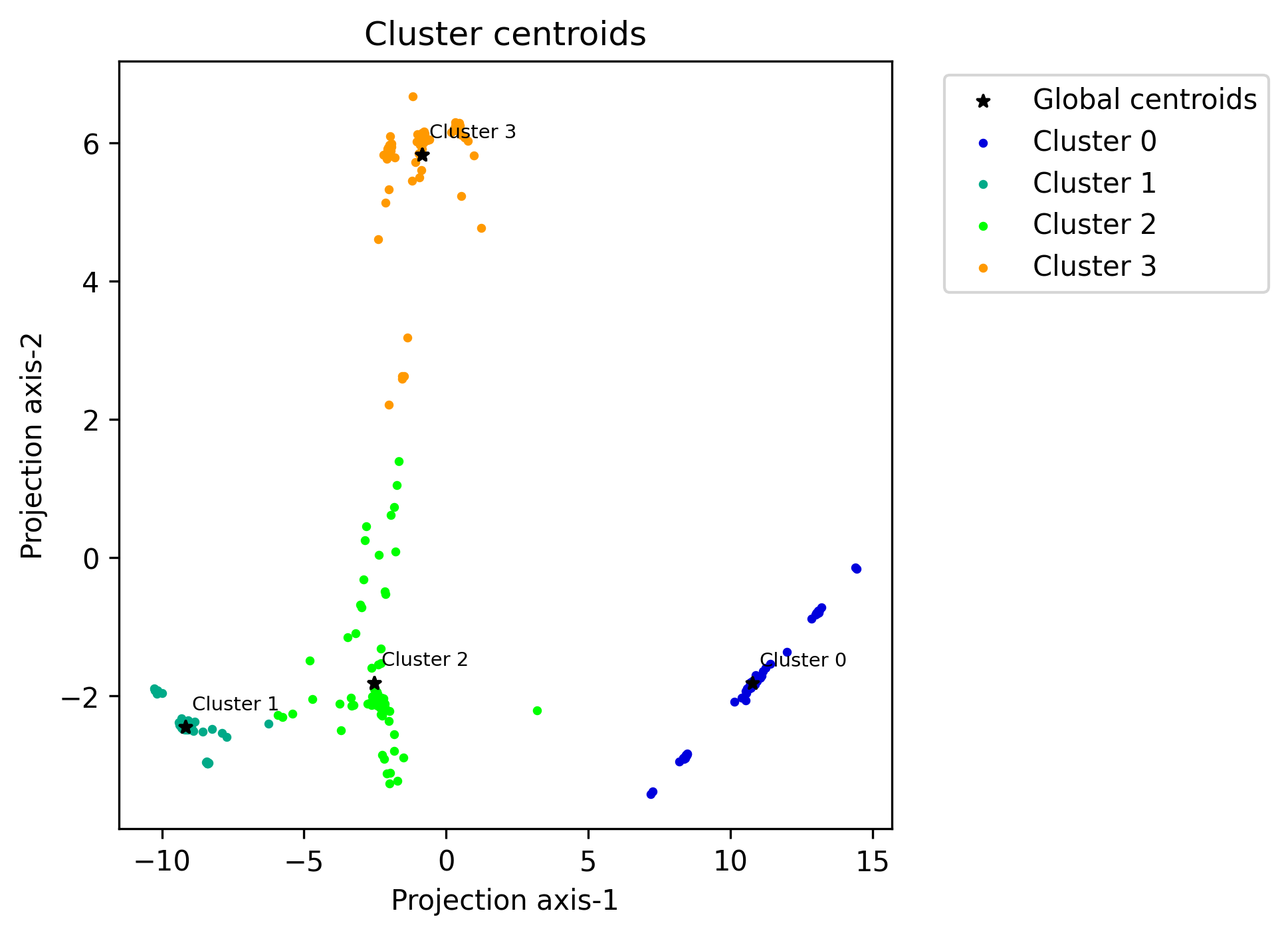
Plot centroids in 2D#
Function: plot_centroids_2d
Global centroids plotted with the local centroids plotted around them. The feature space has been reduced to 2 dimensions using PCA.
- octaipipe.visualization.kfed.plot_centroids_2d(model_id: str, refresh_centroids: bool = True, cluster_label_map: dict = {}, savefig: bool = False, output_path: Optional[str] = None, local_plot_args: dict = {'s': 5}, global_plot_args: dict = {'c': 'black', 'marker': '*', 's': 20}, figsize=(5, 5), plot_title: str = 'Cluster centroids', xlabel: str = 'Projection axis-1', ylabel: str = 'Projection axis-2', annotate_fontsize: int = 7)#
Scatter plot for local and global centroids in 2d-PCA-reduced space.
- Parameters:
model_id (str) – model ID to plot the centroids for.
refresh_centroids (bool) – whether to get centroids from blob storage regardless of whether they are present on machine. Defaults to True
cluster_label_map (dict) – mapping between cluster assignment and label
savefig (bool, optional) – Save figure to file. Defaults to False.
output_path (str, optional) – If savefig is True, must be set to path to save to.
local_plot_args (dict, optional) – plot args for local centroids. Defaults to {‘s’: 5}.
global_plot_args (dict, optional) – plot args for global centroids. Defaults to {‘c’: ‘black’, ‘s’: 10, ‘marker’: ‘*’}.
figsize (tuple, optional) – Defaults to (5, 5).
plot_title (str, optional) – Defaults to ‘Cluster centroids’.
xlabel (str, optional) – Defaults to ‘Projection axis-1’.
ylabel (str, optional) – Defaults to ‘Projection axis-2’.
annotate_fontsize (int, optional) – font size of global centroid annotation. Defaults to 7.
Plot centroids in 3D#
Function: plot_centroids_3d
Global centroids plotted with the local centroids plotted around them. The feature space has been reduced to 3 dimensions using PCA.
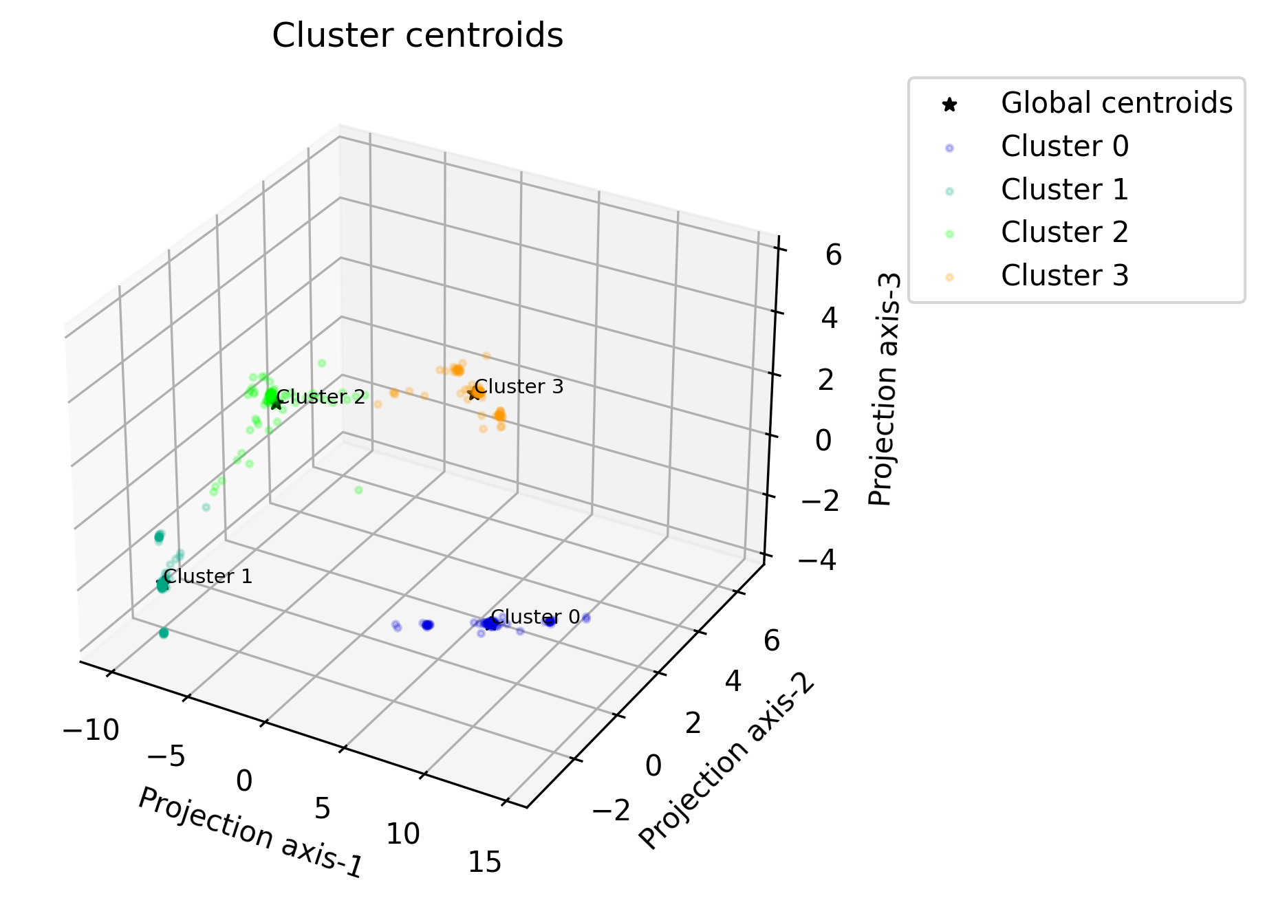
- octaipipe.visualization.kfed.plot_centroids_3d(model_id: str, refresh_centroids: bool = True, cluster_label_map: dict = {}, savefig: bool = False, output_path: Optional[str] = None, local_plot_args: dict = {'alpha': 0.2, 's': 5}, global_plot_args: dict = {'c': 'black', 'marker': '*', 's': 20}, figsize: tuple = (5, 5), plot_title: str = 'Cluster centroids', xlabel: str = 'Projection axis-1', ylabel: str = 'Projection axis-2', zlabel: str = 'Projection axis-3', annotate_fontsize: int = 7)#
Scatter plot for local and global centroids in 3d-PCA-reduced space.
- Parameters:
model_id (str) – model ID to plot the centroids for.
refresh_centroids (bool) – whether to get centroids from blob storage regardless of whether they are present on machine. Defaults to True.
cluster_label_map (dict) – mapping between cluster assignment and label
savefig (bool, optional) – Save figure to file. Defaults to False.
output_path (str, optional) – If savefig is True, must be set to path to save to.
local_plot_args (dict, optional) – plot args for local centroids. Defaults to {‘s’: 5}.
global_plot_args (dict, optional) – plot args for global centroids. Defaults to {‘c’: ‘black’, ‘s’: 10, ‘marker’: ‘*’}.
figsize (tuple, optional) – Defaults to (5, 5).
plot_title (str, optional) – Defaults to ‘Cluster centroids’.
xlabel (str, optional) – Defaults to ‘Projection axis-1’.
ylabel (str, optional) – Defaults to ‘Projection axis-2’.
zlabel (str, optional) – Defaults to ‘Projection axis-3’.
annotate_fontsize (int, optional) – font size of global centroid annotation. Defaults to 7.
Silhouette plot#
Function: silhouette_plot
Plots silhouette values for the local centroids mapped on global clusters. This follows the guide by sklearn
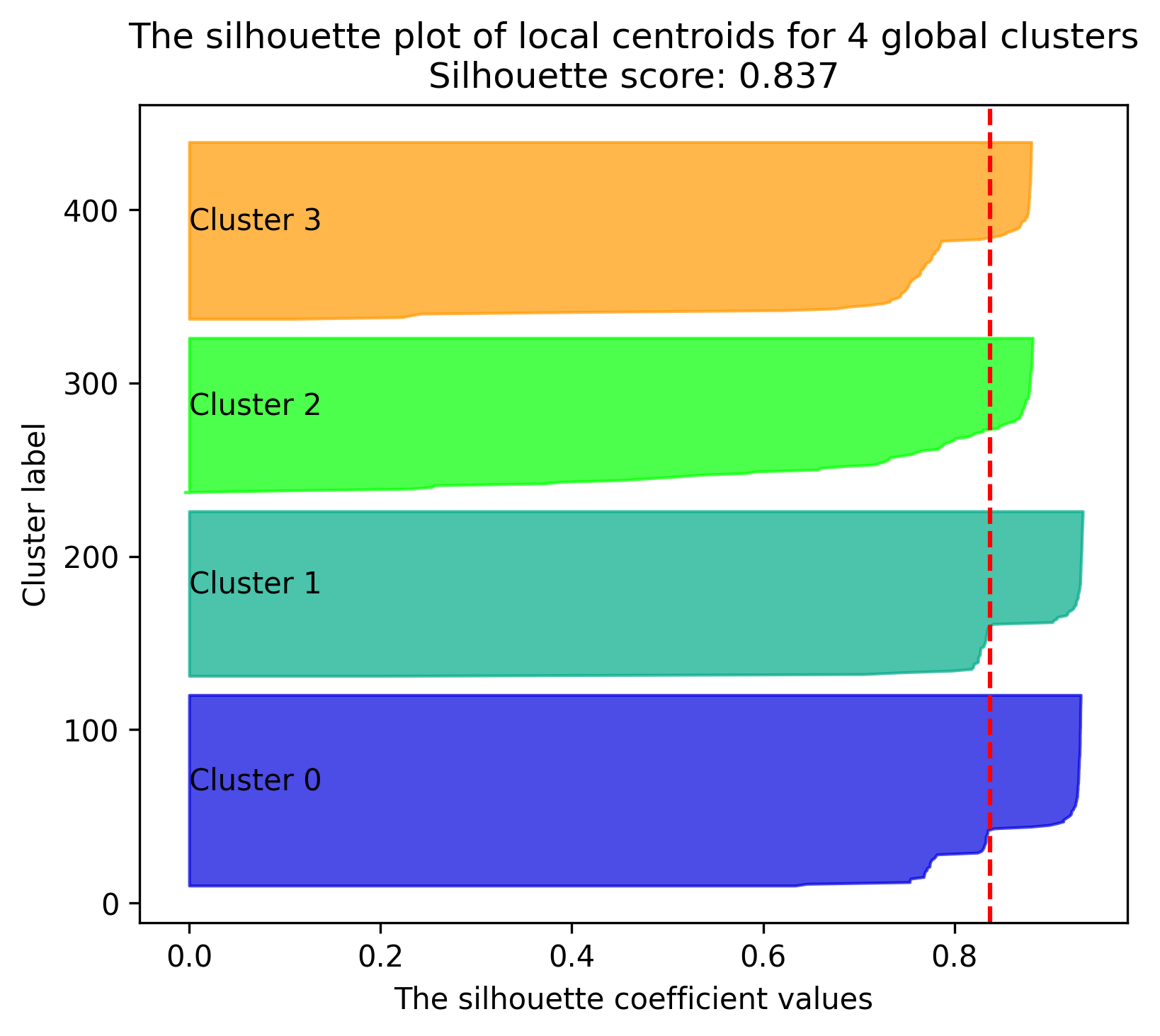
- octaipipe.visualization.kfed.silhouette_plot(model_id: str, refresh_centroids: bool = True, cluster_label_map: dict = {}, savefig: bool = False, output_path: Optional[str] = None, silhouette_score_line_args: dict = {'color': 'red', 'linestyle': '--'}, figsize=(6, 5), plot_title: str = 'The silhouette plot of local centroids', xlabel: str = 'The silhouette coefficient values', ylabel: str = 'Cluster label')#
Silhouette plot for local centroids and global clustering thereof.
- Parameters:
model_id (str) – model ID to plot the centroids for.
refresh_centroids (bool) – whether to get centroids from blob storage regardless of whether they are present on machine. Defaults to True.
savefig (bool, optional) – Save figure to file. Defaults to False.
output_path (str, optional) – If savefig is True, must be set to path to save to.
silhouette_score_line_args (_type_, optional) – plot args for silhouette score line. Defaults to {‘color’: “red”, ‘linestyle’: “–“}.
figsize (tuple, optional) – Defaults to (5, 5).
plot_title (str, optional) – Defaults to ‘The silhouette plot of local centroids’.
xlabel (str, optional) – Defaults to “The silhouette coefficient values”.
ylabel (str, optional) – Defaults to “Cluster label”.
Plot centroid coordinates#
Function: plot_centroids_coordinates
Plots centroid coordinates in feature space. This function as opposed to the other
plotting functions takes the centroids (local or global) as numpy arrays as input
instead of the model_id. To see how to import centroids from file to numpy array,
see the section below.
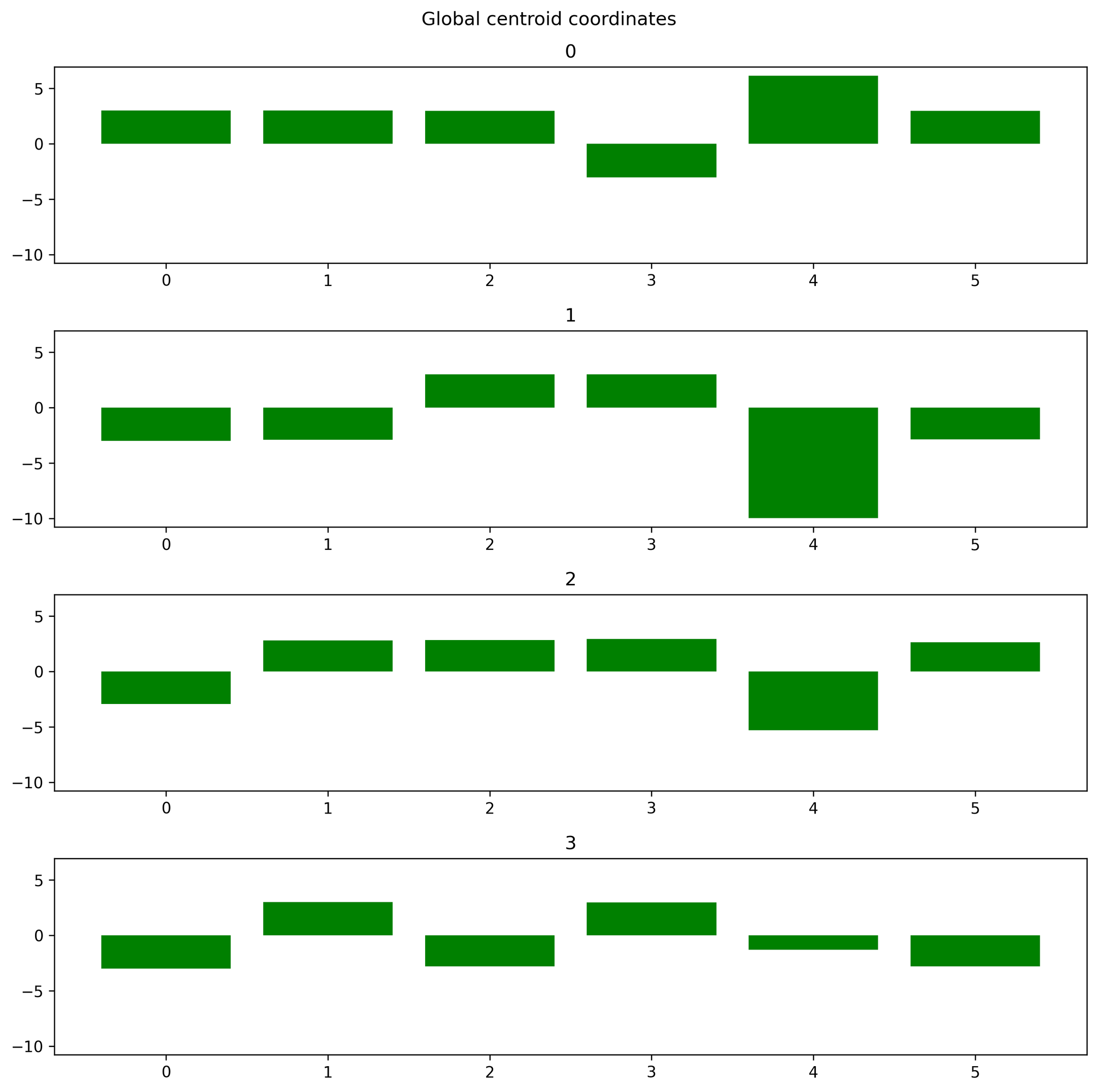
- octaipipe.visualization.kfed.plot_centroids_coordinates(centroids: ndarray[Any, dtype[_ScalarType_co]], cluster_label_map: dict = {}, savefig: bool = False, output_path: Optional[str] = None, figsize: tuple = (10, 10), plot_title: str = 'Global centroid coordinates', plot_args: dict = {'color': 'green'})#
Plot centroid coordinates in bar plot
- Parameters:
centroids (np.typing.NDArray) – centroids to plot coordinates for
cluster_label_map (dict) – mapping between cluster assignment and label
savefig (bool, optional) – Save figure to file. Defaults to False
output_path (str, optional) – If savefig is True, must be set to path to save to.
figsize (tuple, optional) – Defaults to (10, 10).
plot_title (str, optional) – Defaults to ‘Global centroid coordinates’.
plot_args (dict, optional) – Defaults to {‘color’: ‘green’}.
Radar plot#
Function: radar_plot
Plots centroids on radar plot. This function as opposed to the other plotting
functions takes the centroids (local or global) as numpy arrays as input instead of
the model_id. To see how to import centroids from file to numpy array, see the
section below.
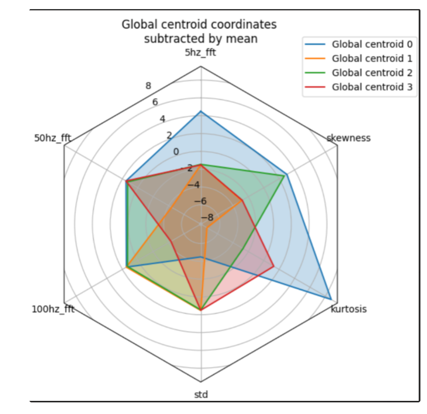
- octaipipe.visualization.kfed.radar_plot(centroids: ndarray[Any, dtype[_ScalarType_co]], cluster_label_map: dict = {}, savefig: bool = False, output_path: Optional[str] = None, figsize: tuple = (10, 10), spoke_labels: Optional[list] = None, plot_title: str = 'Global centroid coordinates \nsubtracted by mean')#
Plots centroids on radar plot showing 5, 50, 100hz frequency spectrum, standard deviation, kurtosis and skew for each centroid.
- Parameters:
centroids (np.typing.NDArray) – centroids to plot coordinates for
cluster_label_map (dict) – mapping between cluster assignment and label
savefig (bool, optional) – Save figure to file. Defaults to False
output_path (str, optional) – If savefig is True, must be set to path to save to.
figsize (tuple, optional) – Defaults to (10, 10).
spoke_labels (Union[list, None], optional) – the labels for the spokes of the radar plot. Should be either None or all feature names in order.
plot_title (str, optional) – Defaults to ‘Global centroid coordinates subtracted by mean’.
Importing centroids from file to numpy array#
To import a centroid from a file to a numpy array, replace {model_id} with your model ID and {centroid_number} with the global centroid number and run the following code:
1import numpy as np
2
3centroid_path = '~/model_metrics/{model_id}/global_centroids/centroid_{centroid_number}.npy'
4
5centroids = np.load(centroid_path)
6centroids: np.typing.NDArray = centroids[centroids.files[0]]
Running k-FED evaluation in OctaiPipe#
Evaluation metrics and centroids are collected for each device and the global k-FED model when the model is trained. However, sometimes, it might be useful to get evaluation metrics for devices not included in training or the same devices but a different dataset.
To help with this, OctaiPipe has an Unsupervised Evaluation step, which runs a k-FED model on a set of devices and adds new local metrics and centroids to the model record.
For example, a user might want to know how well a model created for a set of assets generalizes to a new location. In this case, the user can run the Unsupervised Evaluation step with an esisting model on a new set of devices and compare, amongst other metrics, mean WCSS of the new devices to the existing ones. This gives a quick measure of whether the data distribution on the new assets is similar to the ones on existing assets.
The Unsupervised Evaluation step can be deployed to devices using OctaiPipe’s deploy_to_edge
function. Example code for deploying the step to devices and an example step config is below:
1import logging
2from octaipipe.deployment import deploy_to_edge
3logging.basicConfig(level=logging.INFO, format='%(message)s')
4
5deployment_id = deploy_to_edge(config_path='./configs/deployment_config.yml')
6
7# Once the deployment is finished on the device, run below code
8from octaipipe.deployment import down_deployment
9down_deployment(deployment_id)
Example deployment config#
Filepath: ./configs/deployment_config.yml
name: deployment_config

device_ids: [device-0] # Set device ID(s) to deploy eval to here

image_name: "octaipipe.azurecr.io/octaipipe_lite-all_data_loaders:latest"

env: {}

datasources:
  environment:
   - INFLUX_ORG
   - INFLUX_URL
   - INFLUX_TOKEN

grafana_deployment:
grafana_cloud_config_path:

pipelines:
- unsupervised_evaluation:
      config_path: ./configs/unsupervised_eval.yml
Example Step config#
Filepath: ./configs/unsupervised_eval.yml
name: unsupervised_evaluation

input_data_specs:
  default:
  - datastore_type: influxdb
    settings:
      query_template_path: ./configs/influx_query.txt
      query_type: dataframe
      query_config:
         bucket: test-bucket
         measurement: my-measurement
         start: '2023-01-01T01:00:00.000Z'
         stop: '2023-01-01T05:00:00.000Z'
         tags: {}

model_specs:
  name: kfed_eda_model
  type: kFED
  version: '1'

run_specs:
  target_label: